ISTQB Foundation Level Exam Crash Course Part-11
This is Part 11 of 35 containing 5 Questions (Q. 51 to 55) with detailed explanation as expected in ISTQB Foundation Level Exam Latest Syllabus updated in 2011
Deep study of these 175 questions shall be of great help in getting success in ISTQB Foundation Level Exam
Q. 51: What is the general program structure of a pseudo code?
Code can be of two types, executable and non-executable.
Executable code instructs the computer to take some action; non-executable code is used to prepare the computer to do its calculations but it does not involve any actions.
For example, reserving space to store a calculation (this is called a declaration statement) involves no actions.
In pseudo code non-executable statements will be at the beginning of the program; the start of the executable part is usually identified by BEGIN, and the end of the program by END.
So we get the following structure:
1 Non-executable statements
2 BEGIN
3
4 Executable statements
5
6 END
If we were counting executable statements we would count lines 2, 4 and 6. Line 1 is not counted because it is non-executable. Lines 3 and 5 are ignored because they are blank.
If there are no non-executable statements there may be no BEGIN or END either, but there will always be something separating non-executable from executable statements where both are present.
<<<<<< =================== >>>>>>
Q. 52: In how many ways we can structure the executable code?
Once we have a picture of an overall program structure we can look inside the code. There are only following three ways that executable code can be structured.
1) Sequence: The first is simple & here the statements are exercised one after the other as they appear on the page.
Following is an example of a purely sequential program
1 Read A
2 Read B
3 C = A + B
The BEGIN and END have been omitted in this case since there were no non-executable statements; this is not strictly correct but is common practice, so it is wise to be aware of it and remember to check whether there are any non-executable statements when you do see BEGIN and END in a program. The computer would execute those three statements in sequence, so it would read (input) a value into A (this is just a name for a storage location), then read another value into B, and finally add them together and put the answer into C.
2) Selection: In this case the computer has to decide if a condition (known as a Boolean condition) is true or false. If it is true the computer takes one route, and if it is false the computer takes a different route. Selection structures therefore involve decisions.
Following is an example of a Selection program
1 IF P > 3
2 THEN
3 X = X + Y
4 ELSE
5 X = X − Y
6 ENDIF
Here we ask the computer to evaluate the condition P > 3, which means compare the value that is in location P with 3. If the value in P is greater than 3 then the condition is true; if not, the condition is false. The computer then selects which statement to execute next. If the condition is true it will execute the part labeled THEN, so it executes line 3. Similarly if the condition is false it will execute line 5. After it has executed either line 3 or line 5 it will go to line 6, which is the end of the selection (IF THEN ELSE) structure. From there it will continue with the next line in sequence.
There may not always be an ELSE part, as below:
1 IF P > 3
2 THEN
3 X = X + Y
4 ENDIF
In this case the computer executes line 3 if the condition is true, or moves on to line 4 (the next line in sequence) if the condition is false.
3) Iteration: It simply involves the computer exercising a chunk of code more than once; the number of times it exercises the chunk of code depends on the value of a condition (just as in the selection case).
Iteration structures are called loops. The most common loop is known as a DO WHILE (or WHILE DO) loop and is illustrated below:
1 X = 15
2 Count = 0
3 WHILE X < 20 DO
4 X = X + 1
5 Count = Count + 1
6 END DO
As with the selection structures there is a decision. In this case the condition that is tested at the decision is X < 20. If the condition is true the program �enters the loop� by executing the code between DO and END DO. In this case the value of X is increased by one and the value of Count is increased by one. When this is done the program goes back to line 3 and repeats the test. If X < 20 is still true the program �enters the loop� again. This continues as long as the condition is true. If the condition is false the program goes directly to line 6 and then continues to the next sequential instruction. In the program fragment above the loop will be executed five times before the value of X reaches 20 and causes the loop to terminate. The value of Count will then be 5.
There is another variation of the loop structure known as a REPEAT UNTIL loop. It looks like this:
1 X = 15
2 Count = 0
3 REPEAT
4 X = X + 1
5 Count = Count + 1
6 UNTIL X = 20
The difference from a DO WHILE loop is that the condition is at the end, so the loop will always be executed at least once. Every time the code inside the loop is executed the program checks the condition. When the condition is true the program continues with the next sequential instruction. The outcome of this REPEAT UNTIL loop will be exactly the same as the DO WHILE loop above.
<<<<<< =================== >>>>>>
Q. 53: What is the purpose of creating flow charts?
After we are able to write code we go a step further and create a visual representation of the structure that is much easier to work with. The simplest visual structure to draw is the flow chart, which has only two symbols.
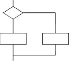
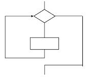
Rectangles represent sequential statements and diamonds represent decisions. More than one sequential statement can be placed inside a single rectangle as long as there are no decisions in the sequence. Any decision is represented by a diamond, including those associated with loops.
To create a flow chart representation of a complete program all we need to do is to connect together all the different bits of structure.
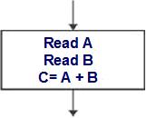
Example of a Flow chart for a sequential program
Example of a Flow chart for a selection (decision) structure
Example of a Flow chart for an iteration (loop) structure
<<<<<< =================== >>>>>>
Q. 54: What is the purpose of making Control Flow Graphs
A control flow graph provides a method of representing the decision points and the flow of control within a piece of code, so it is just like a flow chart except that it only shows decisions. A control flow graph is produced by looking only at the statements affecting the flow of control.
The graph itself is made up of two symbols: 1) Nodes and 2) Edges.
1) A node represents any point where the flow of control can be modified (i.e. decision points), or the points where a control structure returns to the main flow (e.g. END WHILE or ENDIF).
2) An edge is a line connecting any two nodes. The closed area contained within a collection of nodes and edges, as shown in the diagram, is known as a region.
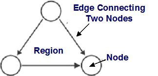
We can draw �sub-graphs� to represent individual structures. For a flow graph the representation of sequence is just a straight line, since there is no decision to cause any branching.
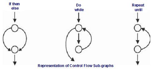
The sub-graphs show what the control flow graph would look like for the program structures we are already familiar with.
<<<<<< =================== >>>>>>
Q. 55: What are the basic steps involved in drawing a control flow graph?
Step-1: Analyze the component to identify all control structures, i.e. all statements that can modify the flow of control, ignoring all sequential statements.
Step-2: Add a node for any decision statement.
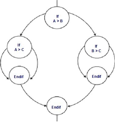
Step-3: Expand the node by substituting the appropriate sub-graph representing the structure at the decision point. Any chunk of code can be represented by using these sub-graphs.
Refer the following example code.
Step 1: breaks the code into statements and identifies the control structures, ignoring the sequential statements, in order to identify the decision points; these are highlighted below.
1 Program MaxandMean
2
3 A, B, C, Maximum: Integer
4 Mean: Real
5
6 Begin
7
8 Read A
9 Read B
10 Read C
11 Mean = (A + B + C)/3
12
13 If A > B
14 Then
15 If A > C
16 Then
17 Maximum = A
18 Else
19 Maximum = C
20 Endif
21 Else
22 If B > C
23 Then
24 Maximum = B
25 Else
26 Maximum = C
27 Endif
28 Endif
29
30 Print (“Mean of A, B and C is “, Mean)
31 Print (“Maximum of A, B, C is “, Maximum)
32
33 End
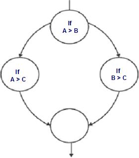
Step 2: Adds a node for each branching or decision statement as shown in following figure.
Step 3: Expands the nodes by substituting the appropriate sub-graphs as shown in following Fugure
Part – 12 of the Crash Course – ISTQB Foundation Exam
Access The Full Database of Crash Course Questions for ISTQB Foundation Level Certification

An expert on R&D, Online Training and Publishing. He is M.Tech. (Honours) and is a part of the STG team since inception.
